When working with real-time streaming data, segmentation will be one of the first issues you encounter. Real-time streaming data has to be carved up into smaller windows for consideration by a machine learning model, and how you carve up that stream can have a major impact on model performance and power consumption. Tune in to the Arm® AI Virtual Tech Talk to learn how you can build effective, low power, low memory sensing applications.
Segmentation: Sliding Windows vs. Triggering
Generally, there are two main ways of doing it:
- Sliding Windows – pass a window of fixed length over the data as it arrives, and use each frame of window contents for training, testing or inference
- Triggered Windows – use thresholds or some other criteria to determine when a window should begin
Sliding windows are by far the easiest and most common way to handle streaming data. They work well in many circumstances after you experiment with window-length and stride (the overlap or distance between subsequent windows). But continuous inference based on sliding windows can be computationally expensive inference. The technique requires that the process run continually, passing each window through the full machine learning evaluation, repeating computations for every window as it is received. This can make a lot of sense for signals in which the target is a subtle variation in a continuous process (such as machine health monitoring), or potentially buried in environmental noise (like a wake word listener). But for detecting and classifying discrete, episodic events, using some kind of triggering can be just as effective and a lot more efficient.
Segmentation and Machine Learning
The typical data flow in a machine learning inference process looks something like this: a) an incoming signal is segmented in some way, b) the contents of each segment are then used for feature computation, c) the resulting feature vector is used as input to the machine learning inference model, generating a result which is then d) smoothed in some way to correct momentary errors.

An example based on deep learning (DL) on sound might look something like this: we start by segmenting the incoming audio stream with, let's say, 250ms windows with 25% overlapping strides (i.e., each subsequent window overlaps the previous one by 25% to ensure we don't miss an event split between windows), compute a Mel-spectrogram on each window, apply a CNN layer to sniff out important time-frequency blobs as features, feed that output into our DL inference network and deliver the result. Even with clever tricks, all those FFTs and filters for the spectrogram, and convolutions and network layers for the DL model add up to a significant amount of active machinery. And this machinery runs all the time, consuming CPU cycles and power even when it's perfectly obvious that there is nothing we care about happening.
If the situation demands, this is powerful stuff. But in many TinyML cases, events are episodic, background noise is sparse, and we are on a tight battery budget.
Wake up!
"Wake up on event" is an old concept in engineering, and is still often employed in hardware solutions. Many accelerometers, embedded microphone chips, and other sensors have a mode in which they sit in a low power state until and unless the energy of a certain level is detected. This can generate an interrupt that wakes upstream hardware in order to react.
The same principle applies in micro-controller-based systems; Arm Cortex-M chips can, for example, be configured to wake up, empty a buffer, perform a quick computation, and go back to sleep. Many systems can sleep or sit at low clock rates until actual horsepower is needed. To take advantage of these power-saving features though, we have to abandon sliding windows and instead look at triggering.
Triggering involves using energy or some other transform derived from the incoming signal. That transform output can then be compared to a threshold, generating a "wake up" event when that threshold is crossed. Other criteria can also be applied – perhaps triggering only when transform output crosses a threshold on the way up or on the way down, for example.
Triggering can also free processors to do other tasks. That DL pipeline is probably a full-time job on most small MPUs and a noticeable thread on a bigger processor, consuming CPU and memory resources that could be used for other work. Perhaps you could squeeze more functionality onto the same hardware if you had those cycles back to use!
How to Use Triggered Segmentation
This kind of approach can be useful for Smart Home — detecting glass breaks, the door opens, dog barks, smoke alarm listeners, presence detection. It could also be usable in automotive — detecting collisions, pot-hole impacts, vandalism, etc. Or perhaps in smart devices, quietly waiting in low power mode for something to act on. Any application where you are looking for discrete events that happen occasionally, rather than monitoring a continuous process is a candidate.
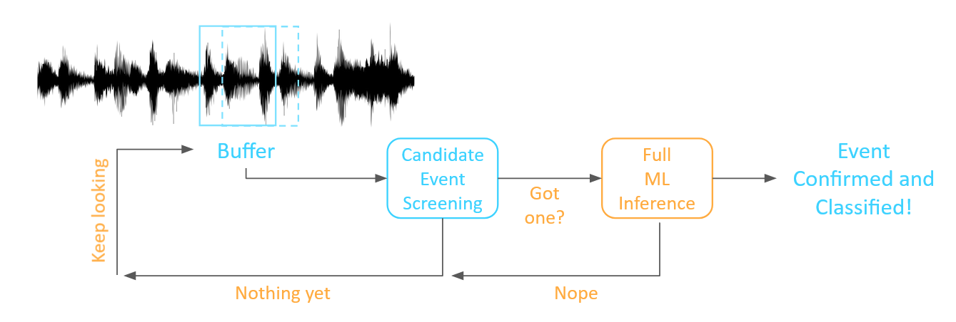
This approach is really a special case of a more general, two-stage AI architecture. In this architecture, some form of low-resource screening method is employed continuously, monitoring the contents of the input buffer. When a triggering threshold is crossed, a candidate window of data is passed to the machine learning inference model, which then evaluates and classifies it. In this architecture, that full inference model only runs when something has happened that makes us think that a target event may have occurred – consuming fewer computational resources and much less power.

The trick, of course, is to make the screening step computationally lightweight, while still rejecting as many true negatives as possible.
If the environment is basically quiet, we might choose to evaluate any signal window with an RMS energy above a predefined threshold. We can even dynamically adjust that threshold based on average noise levels in recent history. But we can get more creative and still remain computationally light.
Hardware engineers will think about the controls for setting up an oscilloscope trigger: looking for positive-going or negative-going threshold crossings, or looking at sums or differences of channels are all fast, low computation screening triggers (and all are supported in Reality AI Tools software for creating Edge AI/TinyML models). Another mechanism I find useful is detecting a sudden step in RMS energy, either a transient event or a transient dip compared to whatever background noise is present. With just a small amount of computation, we can also consider filtering the incoming signal and looking at energy in specific frequency bands rather than over the entire range.
A critical detail for practitioners of AI, however, is that the two layers of this architecture interact significantly. The Full ML layer needs to be optimized to make decisions specifically on candidates that pass screening to distinguish True from False positives. This means the training set must reflect what the segmentation logic will output and the detector will see in deployment. It also means that the ML layer can often be much simpler than would otherwise be required.
In the next installment, we will discuss how software like Reality AI Tools can help you design and implement an effective triggering mechanism, lowering the computational intensity, power consumption of your Edge AI system.


